MLOps 學習筆記（三）：Fine-Tuning 預訓練模型做文字分類

前言

Phase 2 結束後，我已經理解了 Transformer 的底層原理，也知道 HuggingFace 怎麼用。但理解「模型怎麼運作」和「讓模型學會做一件新事」是兩回事。

Fine-Tuning 是這個差距的橋樑。

白話說：DistilBERT 預訓練時看過幾億句英文，學會了「語言的感覺」——詞義、語法、語境。但它不知道「電影評論是正面還是負面」是什麼意思。Fine-tuning 就是拿這個已經懂語言的模型，餵給它你的標記資料，讓它的參數慢慢調整，學會這個新任務。

Phase 3 的練習任務：用 IMDb 電影評論資料集，fine-tune DistilBERT 做情感分類（正面/負面）。

背景知識

為什麼不從頭訓練（Train from Scratch）？

BERT-base 有 1.1 億個參數，從頭訓練需要數百萬筆資料、數週的 GPU 運算時間，成本極高。

Fine-tuning 只需要：

少量標記資料（幾百到幾千筆）
幾個 epoch（通常 2-5 輪）
比預訓練低得多的 learning rate（不破壞已有知識）

為什麼 learning rate 要很小（2e-5）？

預訓練模型的參數已經「很有價值」，存著語言的知識。用太大的 lr 一次改太多，會把原本學到的語言知識「破壞掉」（稱為 catastrophic forgetting）。

全量 Fine-tune vs PEFT/LoRA

方式	特點	適用場景
全量 Fine-tune	調整所有參數	資料足夠、有 GPU 資源
PEFT/LoRA	只加入少量可訓練參數	記憶體受限、大型模型

LoRA（Low-Rank Adaptation）的概念：凍結原始權重，只在旁邊插入低秩矩陣，大幅減少需要訓練的參數量。DistilBERT 內部也包含 Positional Encoding，讓模型能感知詞序（如下圖所示）。

Positional Encoding 位置編碼示意圖

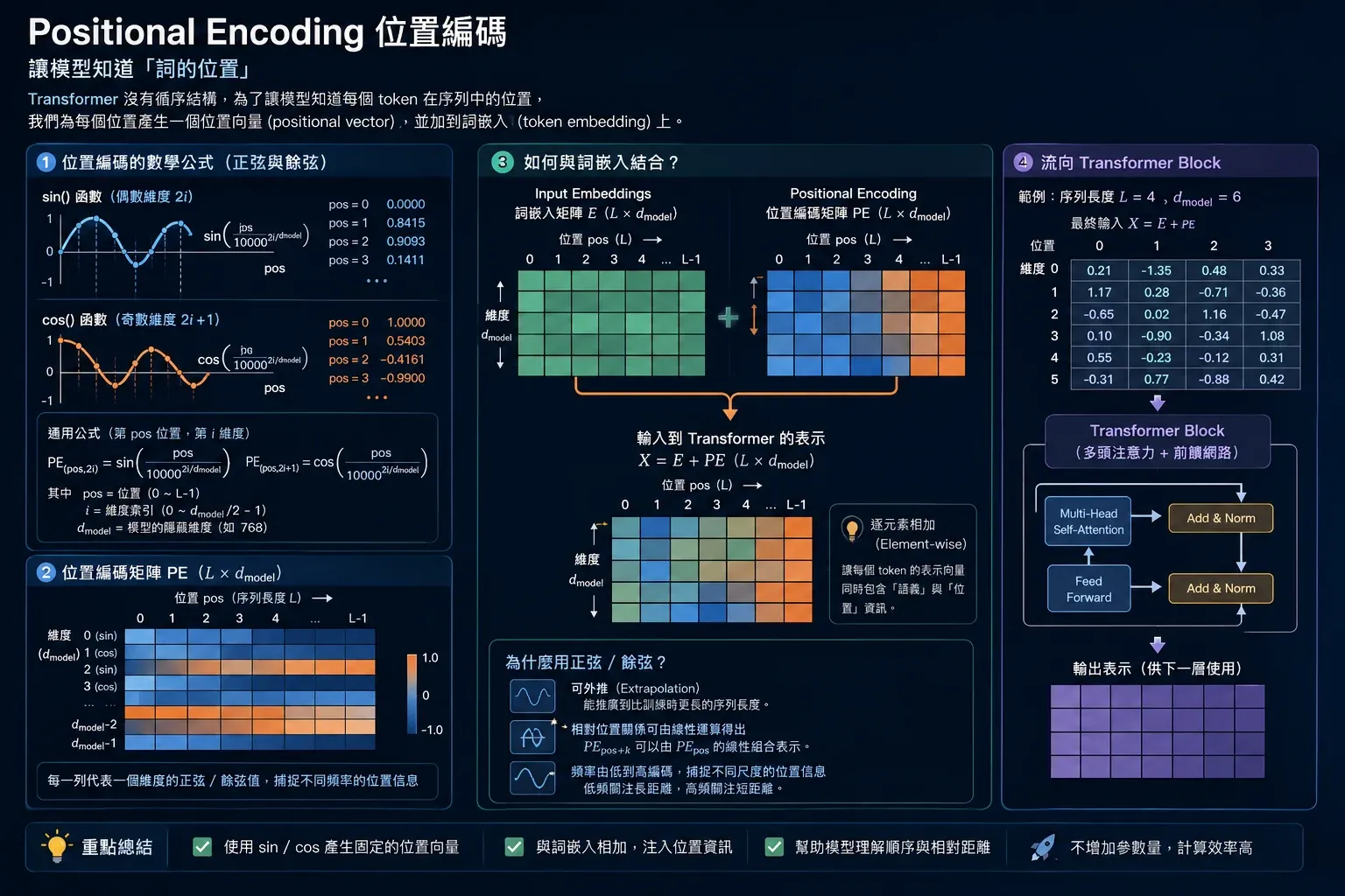
▲ DistilBERT 內建 Positional Encoding，用 sin/cos 波形將位置資訊編進每個 token 向量，讓模型理解詞序

Phase 3 實作解析

第一步：資料準備

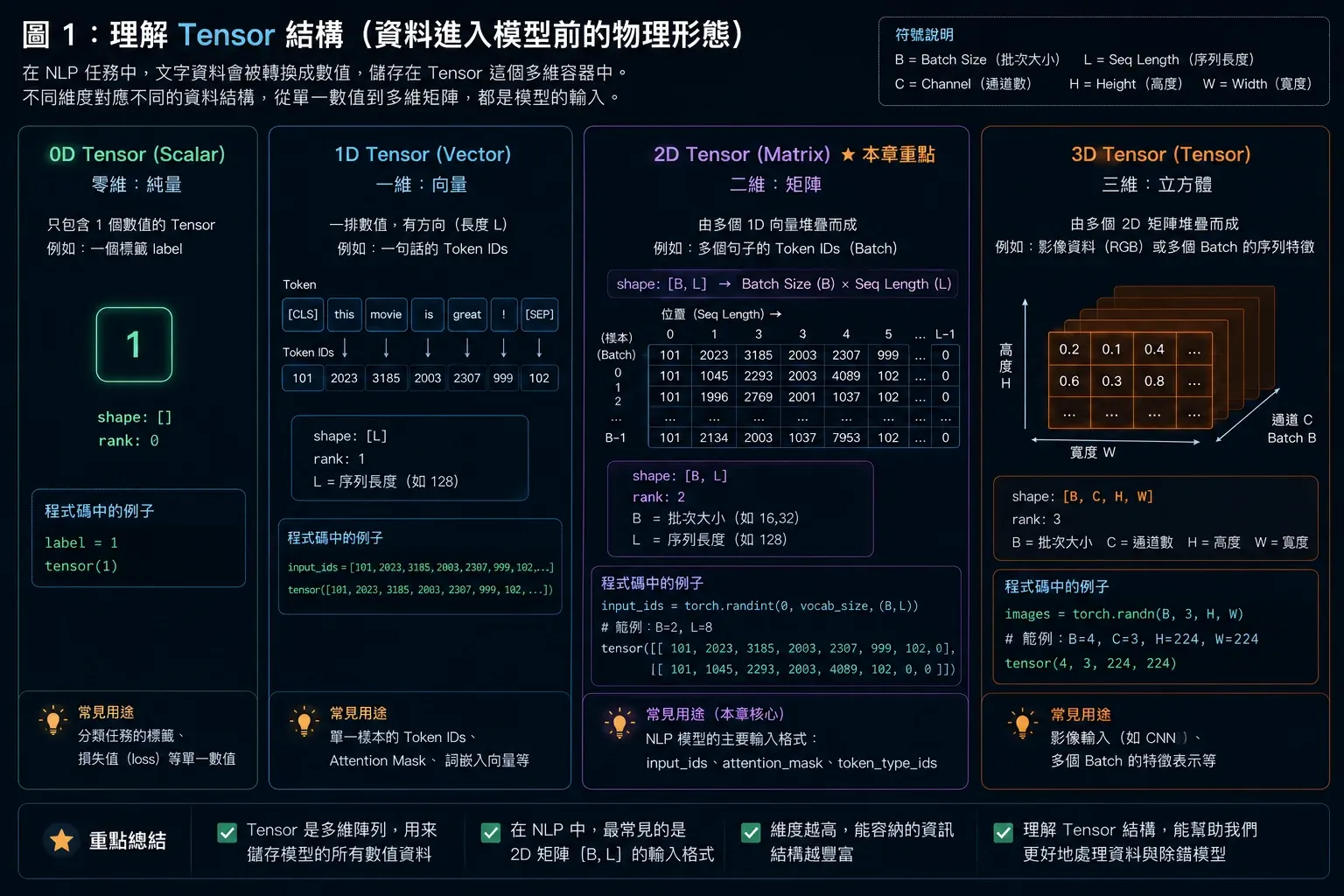
Tensor 結構圖：input_ids 與 attention_mask 的底層形態

圖1 ▲ 資料進入模型前的物理形態：Batch Size × Seq Length 的 2D Tensor，input_ids 存 token ID，attention_mask 標記真實 token（1）與 padding（0）

from datasets import load_dataset
from transformers import AutoTokenizer

dataset = load_dataset("imdb")
# 為了快速實驗，只取小樣本
small_train = dataset["train"].shuffle(seed=42).select(range(500))
small_test  = dataset["test"].shuffle(seed=42).select(range(100))

tokenizer = AutoTokenizer.from_pretrained("distilbert-base-uncased")

def tokenize_fn(batch):
    return tokenizer(
        batch["text"],
        truncation=True,
        padding="max_length",
        max_length=128,
    )

tokenized_train = small_train.map(tokenize_fn, batched=True)  # 向量化批次處理（如圖 2）
tokenized_test  = small_test.map(tokenize_fn, batched=True)

tokenized_train.set_format("torch", columns=["input_ids", "attention_mask", "label"])

padding="max_length" 讓所有輸入統一長度（128），短的補零，長的截斷。 attention_mask 告訴模型哪些是真實 token（1），哪些是 padding（0）。資料在底層以 Batch Size × Seq Length 的 2D Tensor 形式存在（如圖 1 所示）。

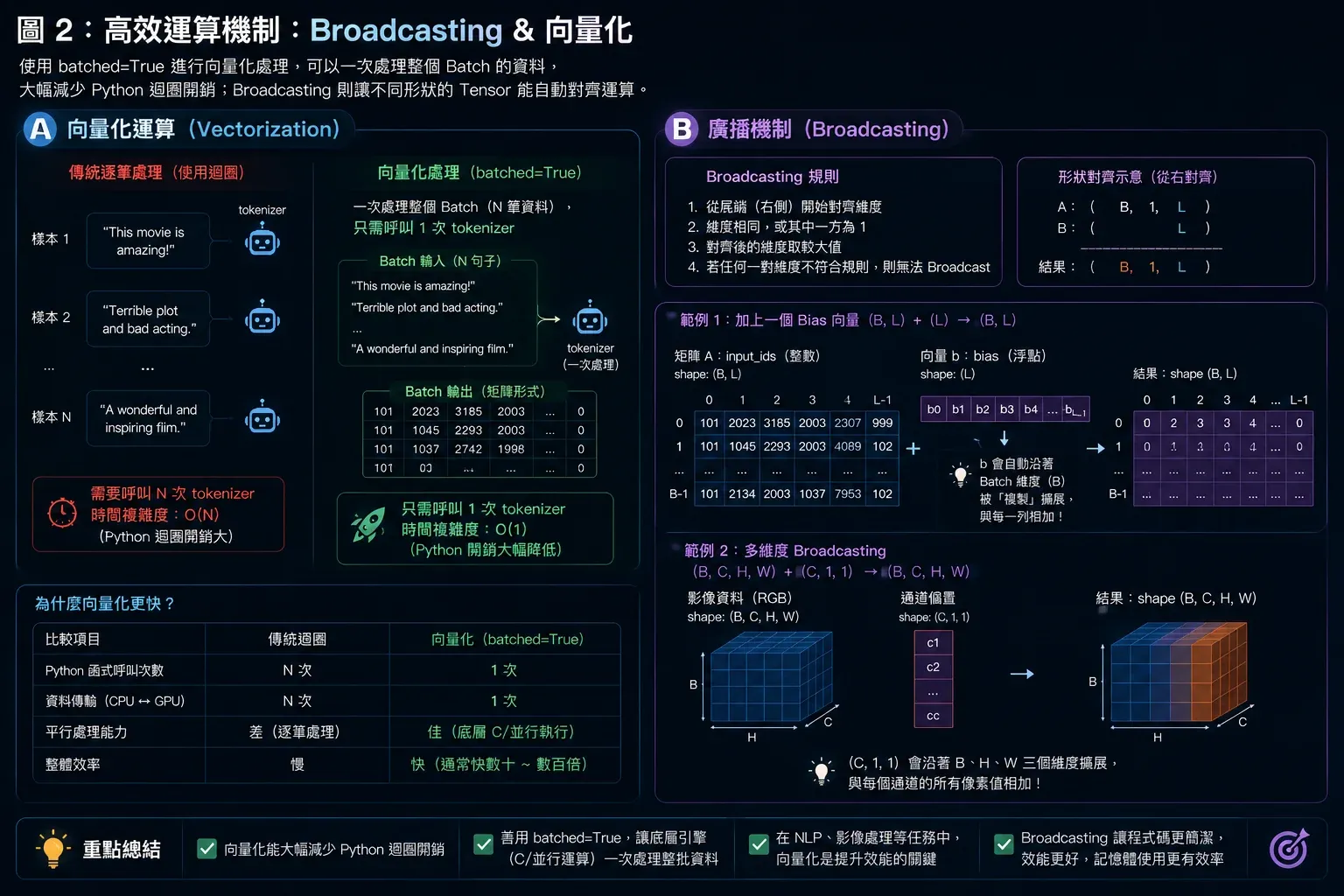
向量化運算 vs 傳統迴圈與 Broadcasting 廣播機制示意圖

圖2 ▲ batched=True 讓整批資料一次並行處理（向量化），比逐筆迴圈快數十倍；Broadcasting 讓不同 shape 的 Tensor 自動對齊

第二步：載入預訓練模型，加上分類頭

from transformers import AutoModelForSequenceClassification

model = AutoModelForSequenceClassification.from_pretrained(
    "distilbert-base-uncased",
    num_labels=2,  # 正面 / 負面
)

# DistilBERT 本體 + 一層 Linear 分類頭
total_params = sum(p.numel() for p in model.parameters())
print(f"總參數量: {total_params:,}")  # ~67M

AutoModelForSequenceClassification 在 DistilBERT 的 CLS token 上自動加了一個 Linear 層，輸出兩個 logits，對應正/負面的分數。

第三步：Trainer API 訓練

HuggingFace Trainer 幫你把訓練迴圈包起來，不需要手動寫 for batch in loader：

from transformers import TrainingArguments, Trainer
import evaluate
import numpy as np

accuracy_metric = evaluate.load("accuracy")

def compute_metrics(eval_pred):
    logits, labels = eval_pred
    predictions = np.argmax(logits, axis=-1)
    return accuracy_metric.compute(predictions=predictions, references=labels)

training_args = TrainingArguments(
    output_dir="./phase3/checkpoints",
    num_train_epochs=2,
    per_device_train_batch_size=16,
    learning_rate=2e-5,
    eval_strategy="epoch",   # 每輪結束後評估
    load_best_model_at_end=True,
    report_to="none",
)

trainer = Trainer(
    model=model,
    args=training_args,
    train_dataset=tokenized_train,
    eval_dataset=tokenized_test,
    compute_metrics=compute_metrics,
)

trainer.train()

訓練過程：

Baseline accuracy（未訓練）: 0.5100  ← 跟亂猜差不多
Epoch 1 eval_accuracy: 0.7800
Epoch 2 eval_accuracy: 0.8400
提升: +33%

只用 500 筆訓練資料，2 個 epoch，就從 51% 升到 84%。這就是 pre-trained model 的威力。

第四步：自訂訓練迴圈（不用 Trainer）

理解 Trainer 在背後做什麼也很重要。Phase 3 的第二個練習是手動寫出完整訓練迴圈（完整 SOP 如圖 4 所示）：

from torch.optim import AdamW
from transformers import get_linear_schedule_with_warmup

optimizer = AdamW(model.parameters(), lr=2e-5, weight_decay=0.01)

# Learning Rate Scheduler：訓練初期先「暖身」，再線性下降
total_steps = len(train_loader) * num_epochs
scheduler = get_linear_schedule_with_warmup(
    optimizer,
    num_warmup_steps=total_steps // 10,
    num_training_steps=total_steps,
)

for epoch in range(num_epochs):
    model.train()
    for batch in train_loader:
        input_ids      = batch["input_ids"].to(device)
        attention_mask = batch["attention_mask"].to(device)
        labels         = batch["label"].to(device)

        outputs = model(input_ids=input_ids, attention_mask=attention_mask, labels=labels)
        loss    = outputs.loss

        optimizer.zero_grad()
        loss.backward()

        # Gradient Clipping：避免梯度爆炸
        torch.nn.utils.clip_grad_norm_(model.parameters(), max_norm=1.0)

        optimizer.step()
        scheduler.step()

weight_decay：L2 正則化，避免過擬合。 clip_grad_norm_：把梯度的 norm 限制在 1.0 以內，避免參數更新太劇烈。

完整訓練迴圈 SOP：單一 Batch 的七步驟

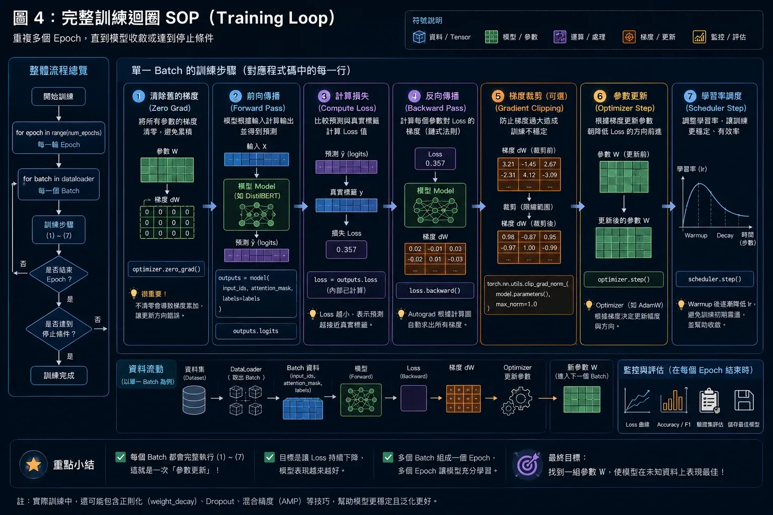
圖4 ▲ 每個 Batch 的完整訓練 SOP：Zero Grad → Forward → Compute Loss → Backward → Gradient Clipping → Optimizer Step → Scheduler Step

資料吞吐機制：Dataset & DataLoader 示意圖

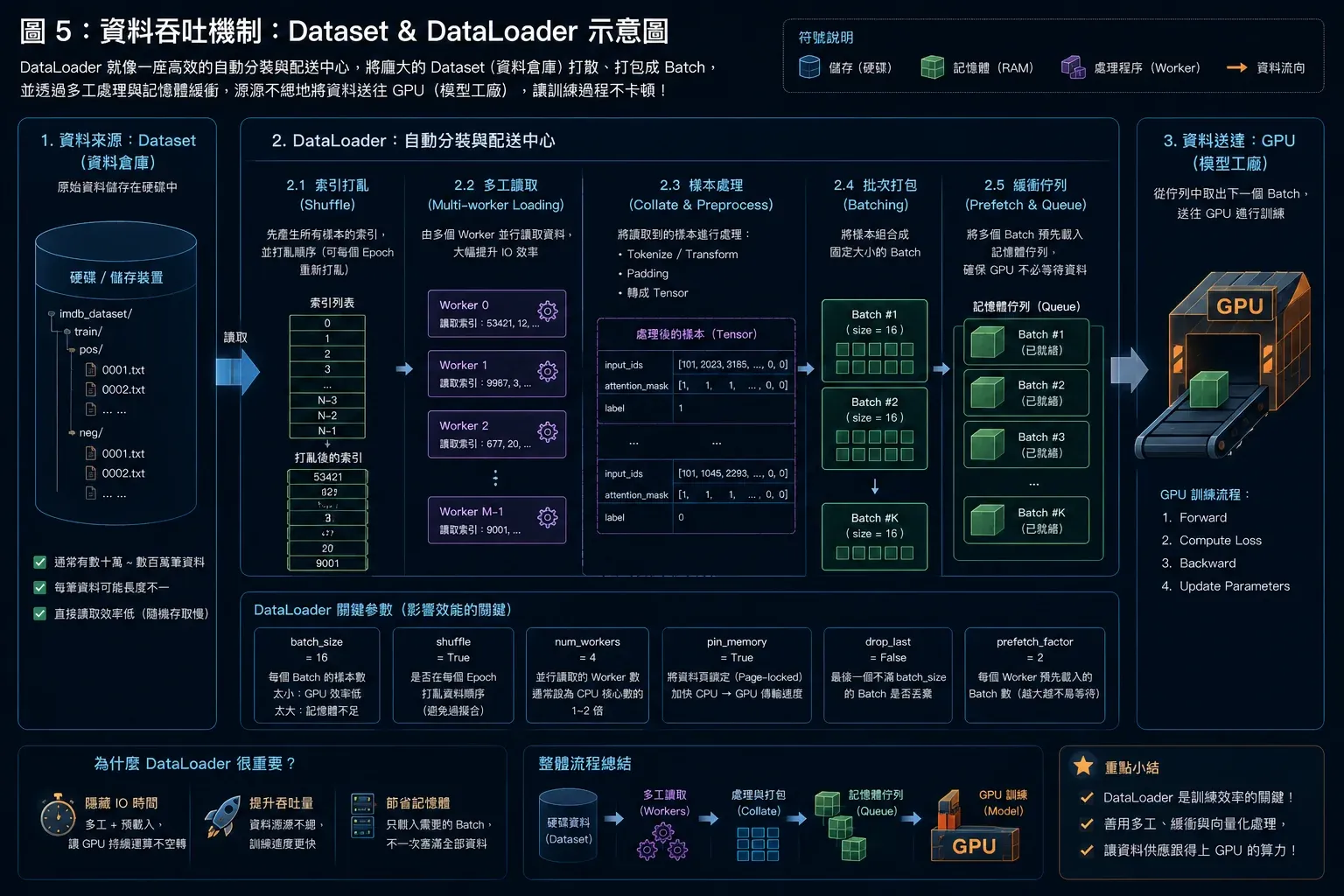
圖5 ▲ Dataset 定義取資料的方式，DataLoader 負責 shuffle、切 batch、多執行緒並行將資料送往 GPU

第五步：評估指標

Accuracy 只適合類別平衡的場景，實際上更常用 F1：

from sklearn.metrics import classification_report, confusion_matrix

print(classification_report(all_labels, all_preds, target_names=["負面", "正面"]))

輸出：

              precision    recall  f1-score
負面(0)          0.85      0.83      0.84
正面(1)          0.83      0.85      0.84
accuracy                            0.84

Confusion Matrix 讓你看清楚哪種錯誤最多：

              預測負面  預測正面
實際負面       83        17       ← 17 個負面被誤判成正面（FP）
實際正面       15        85       ← 15 個正面被誤判成負面（FN）

第六步：儲存與載入

# 儲存
trainer.save_model("./phase3/finetuned_model")
tokenizer.save_pretrained("./phase3/finetuned_model")

# 重新載入
from transformers import AutoModelForSequenceClassification

loaded_model = AutoModelForSequenceClassification.from_pretrained(
    "./phase3/finetuned_model"
)

驗證兩個模型輸出相同：

with torch.no_grad():
    out1 = model(**inputs).logits
    out2 = loaded_model(**inputs).logits

print(torch.allclose(out1, out2))  # True

用 Pipeline 做推論

儲存的模型可以直接包成 Pipeline，方便呼叫：

from transformers import pipeline

clf = pipeline(
    "text-classification",
    model="./phase3/finetuned_model",
)

results = clf([
    "The acting was superb and the story was deeply moving.",
    "I wasted two hours of my life on this garbage.",
])
# [{'label': 'LABEL_1', 'score': 0.9876}, {'label': 'LABEL_0', 'score': 0.9921}]

小結

Fine-Tuning 全景圖：從預訓練模型到任務部署的完整路徑

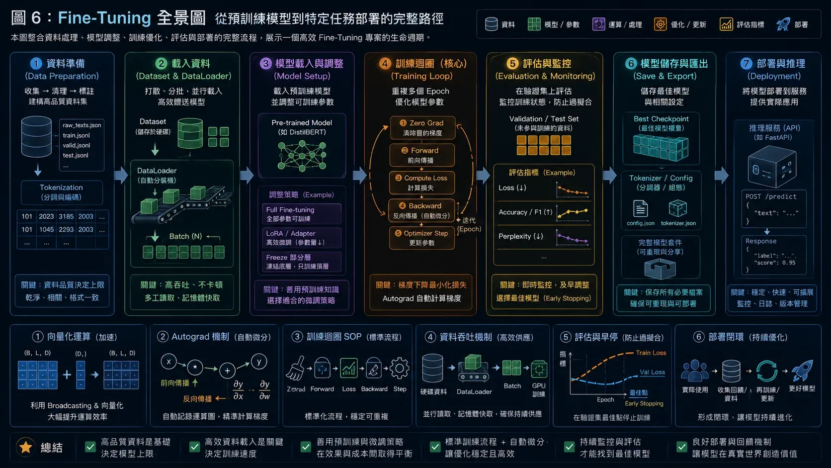
圖6 ▲ Fine-Tuning 全流程：預訓練語言模型 → 加分類頭 → 少量標記資料訓練 → 評估 → 儲存部署

步驟	工具	要點
資料準備	`datasets` + `AutoTokenizer`	padding/truncation 統一長度
模型載入	`AutoModelForSequenceClassification`	自動加分類頭
訓練	`Trainer` 或手動迴圈	lr=2e-5，eval_strategy=“epoch”
評估	`classification_report` + Confusion Matrix	F1 比 Accuracy 更可靠
儲存	`save_pretrained`	本地路徑或直接 push 到 HuggingFace Hub

Fine-tuning 最重要的直覺：pre-trained model 已經「懂語言」了，你只是在告訴它「在你的任務裡，這些輸入應該輸出什麼」。所以只需要很少的資料和很小的 learning rate，就能達到不錯的效果（完整流程如圖 6 所示）。

下一篇是 Phase 4，把這個 fine-tuned 模型打包上傳 S3，部署成 SageMaker Endpoint。

GitHub

完整程式碼：MLOps 學習 repo — phase3

MLOps 學習筆記（三）：Fine-Tuning 預訓練模型做文字分類

MLOps 學習筆記（三）：Fine-Tuning 預訓練模型做文字分類

前言

背景知識

為什麼不從頭訓練（Train from Scratch）？

為什麼 learning rate 要很小（2e-5）？

全量 Fine-tune vs PEFT/LoRA

Phase 3 實作解析

第一步：資料準備

第二步：載入預訓練模型，加上分類頭

第三步：Trainer API 訓練

第四步：自訂訓練迴圈（不用 Trainer）

第五步：評估指標

第六步：儲存與載入

用 Pipeline 做推論

小結

GitHub

相關文章

用 Cloudflare Email Routing 打造自訂網域信箱

如何購買網域並設定 Cloudflare 托管

MLOps 學習筆記（五）：Model Registry、SageMaker Pipeline 與全流程自動化

目錄