前言

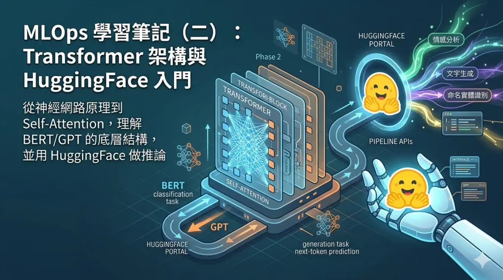
學完 Phase 1 的訓練迴圈之後，我開始思考一個問題：GPT 和 BERT 這類大語言模型，和我訓練的線性迴歸在結構上有什麼本質差異？

答案是 Transformer 架構，而核心是 Self-Attention 機制。

這個機制解決了一個語言處理的根本問題：「處理一個詞的時候，要怎麼知道句子裡其他詞對它的影響？」

以「銀行旁邊有條河」和「我去銀行存錢」為例，「銀行」這個詞出現在完全不同的語境，意思不同。傳統的 RNN 會順序處理，很難捕捉長距離依賴；Self-Attention 讓每個詞能同時「看到」整個句子，動態決定關注哪些詞。

---

背景知識

神經網路的核心三步驟

步驟	說明
Forward Pass（前向傳播）	資料從輸入層流向輸出層，得到預測值
Loss Function	衡量預測和真實的差距（CrossEntropy、MSE）
Backpropagation（反向傳播）	用 chain rule 從輸出往回算每個參數的梯度

Activation Function 為什麼重要？

如果沒有 activation function，不管疊幾層線性層，整個網路等價於一層線性變換，沒辦法學習非線性關係：

沒有 activation：Linear → Linear → Linear ≡ 一個 Linear
有 activation：Linear → ReLU → Linear → ReLU → Linear（真正的深度網路）

ReLU 是最常用的選擇：簡單、計算快、梯度不容易消失：

$\text{ReLU}(x) = \max(0, x)$

Transformer 的核心：Q、K、V

Self-Attention 把每個 token 轉成三個向量：

• Q（Query）：「我想找什麼資訊？」
• K（Key）：「我有什麼資訊？」
• V（Value）：「我實際提供的內容」

計算流程：Q 和每個 K 做內積 → Softmax 得到注意力權重 → 對 V 做加權平均（如圖 1 所示）：

$\text{Attention}(Q, K, V) = \text{softmax}\!\left(\frac{QK^\top}{\sqrt{d_k}}\right)V$

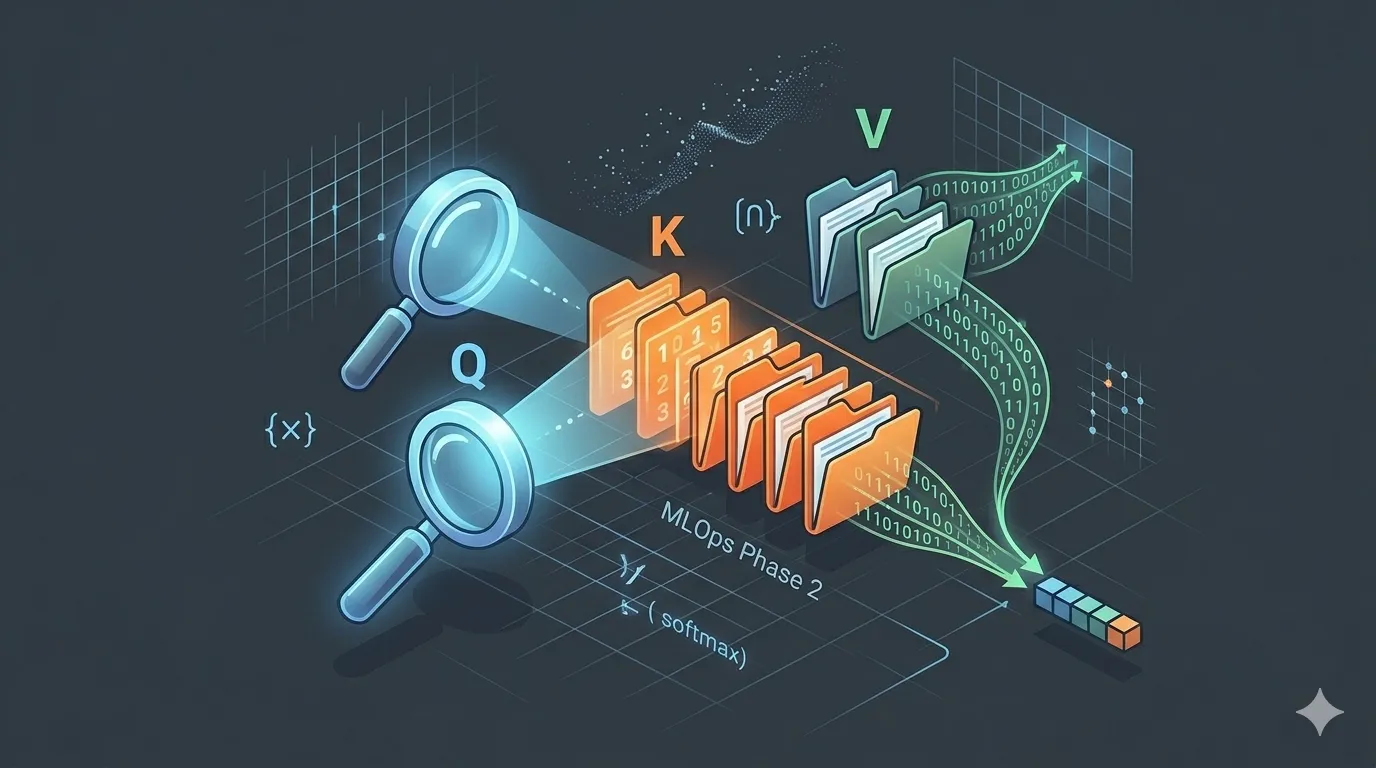
圖1 ▲ Q（放大鏡）對準每個 K（文件夾）做配對，配對權重決定從 V（數據流）中提取多少資訊

---

Phase 2 實作解析

手動實作 Scaled Dot-Product Attention

import torch
import torch.nn.functional as F
import math

def scaled_dot_product_attention(Q, K, V, mask=None):
    """
    Q, K, V: (batch, seq_len, d_k)
    """
    d_k = Q.shape[-1]

    # Q @ K^T：計算每對 token 的相關性分數
    scores = Q @ K.transpose(-2, -1) / math.sqrt(d_k)
    # 除以 sqrt(d_k) 避免內積值太大導致 Softmax 梯度消失

    if mask is not None:
        scores = scores.masked_fill(mask == 0, float('-inf'))

    # Softmax → 每列加總為 1 的注意力權重
    attn_weights = F.softmax(scores, dim=-1)

    # 加權平均 V
    return attn_weights @ V, attn_weights

為什麼要除以 $\sqrt{d_k}$？當維度很高時，內積的值會很大，Softmax 後梯度幾乎消失（某一個位置的權重趨近 1，其他趨近 0），縮放是為了保持梯度穩定。

Multi-Head Attention：同時從多個角度理解

單一 Attention 只能關注一種關係。Multi-Head 讓模型同時從多個角度做 Attention，最後合併（架構如圖 2 所示）：

class MultiHeadAttention(nn.Module):
    def __init__(self, d_model, num_heads):
        super().__init__()
        self.d_k = d_model // num_heads
        self.num_heads = num_heads

        self.W_q = nn.Linear(d_model, d_model)
        self.W_k = nn.Linear(d_model, d_model)
        self.W_v = nn.Linear(d_model, d_model)
        self.W_o = nn.Linear(d_model, d_model)

    def split_heads(self, x):
        batch, seq, _ = x.shape
        # (batch, seq, d_model) → (batch, heads, seq, d_k)
        return x.view(batch, seq, self.num_heads, self.d_k).transpose(1, 2)

    def forward(self, x, mask=None):
        Q = self.split_heads(self.W_q(x))
        K = self.split_heads(self.W_k(x))
        V = self.split_heads(self.W_v(x))

        out, _ = scaled_dot_product_attention(Q, K, V, mask)

        # 合併所有 head → (batch, seq, d_model)
        out = out.transpose(1, 2).contiguous().view(x.shape[0], -1, d_model)
        return self.W_o(out)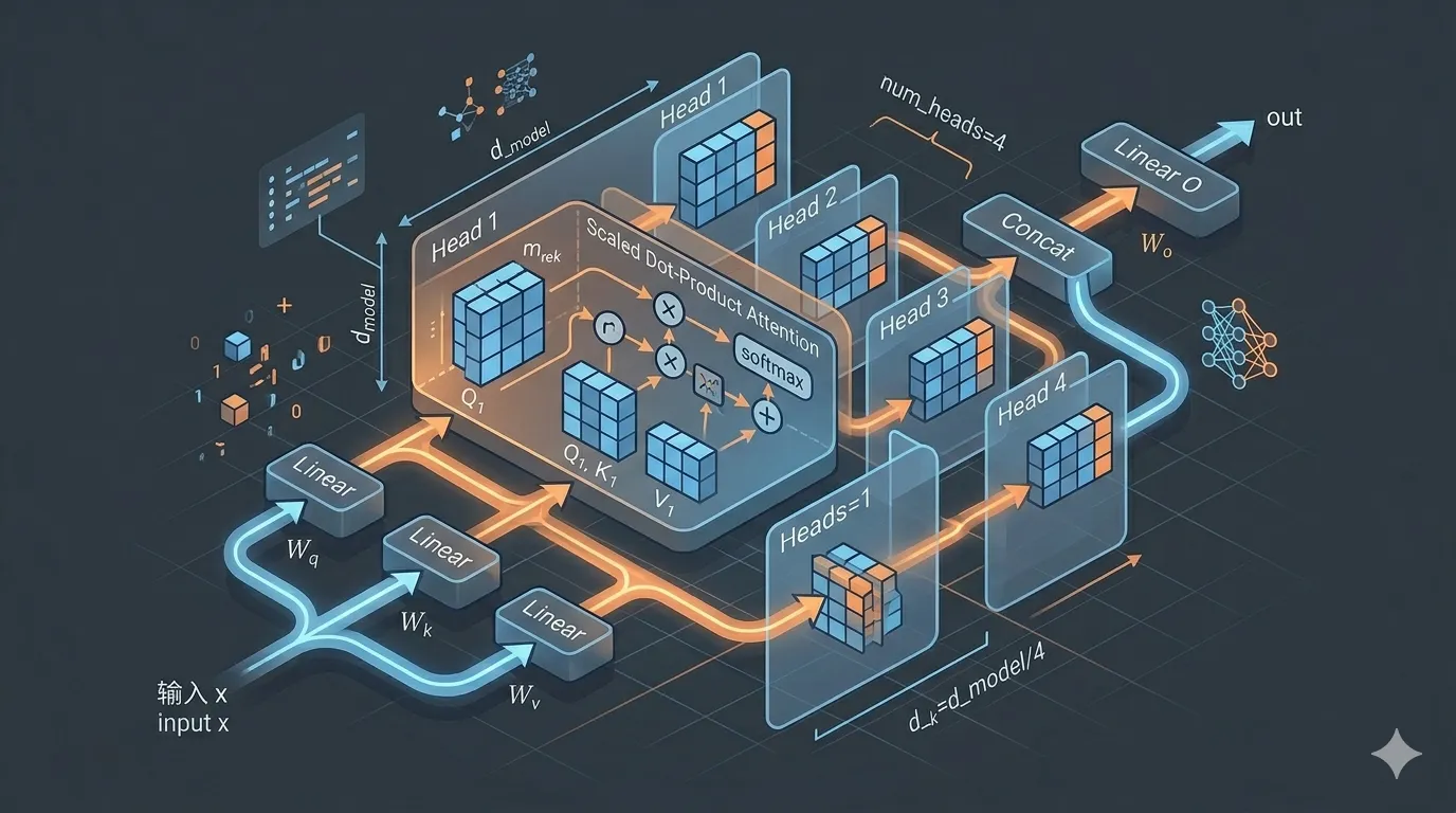

圖2 ▲ Input 經 Linear 投影後分流至多個 Head 各自計算 Attention，最後 Concat 合併輸出

每個 Head 可以關注不同的語言關係：

• Head 1：主詞-動詞關係
• Head 2：指代關係（「他」→「John」）
• Head 3：位置鄰近關係

Positional Encoding：補充順序資訊

Attention 本身沒有「順序」的概念，「我打你」和「你打我」對 Attention 來說看起來一樣。Positional Encoding 用 sin/cos 函式把位置資訊編進向量（如圖 3 所示）：

$PE_{(pos,\ 2i)} = \sin\!\left(\frac{pos}{10000^{2i/d_{\text{model}}}}\right), \quad PE_{(pos,\ 2i+1)} = \cos\!\left(\frac{pos}{10000^{2i/d_{\text{model}}}}\right)$

其中 $pos$ 是 token 在句子中的位置，$i$ 是向量的維度索引。

class PositionalEncoding(nn.Module):
    def __init__(self, d_model, max_len=512):
        super().__init__()
        pe = torch.zeros(max_len, d_model)
        position = torch.arange(0, max_len).unsqueeze(1).float()
        div_term = torch.exp(
            torch.arange(0, d_model, 2).float() * (-math.log(10000.0) / d_model)
        )
        pe[:, 0::2] = torch.sin(position * div_term)  # 偶數維度
        pe[:, 1::2] = torch.cos(position * div_term)  # 奇數維度
        self.register_buffer('pe', pe.unsqueeze(0))

    def forward(self, x):
        return x + self.pe[:, :x.size(1)]  # 加到輸入上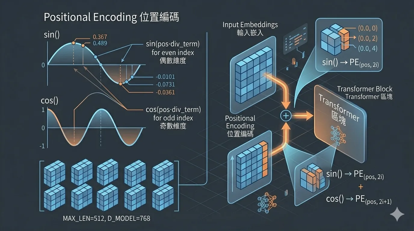

圖3 ▲ 用 sin/cos 波形將位置資訊編進向量，讓模型區分「我打你」與「你打我」的詞序差異

BERT vs GPT：Encoder vs Decoder

	BERT	GPT
架構	Encoder Only	Decoder Only
方向	雙向（看整句話）	單向（只看左邊）
預訓練任務	Masked Language Model	Next Token Prediction
適合任務	分類、NER、問答	文字生成

兩種架構的設計差異如圖 4 所示。

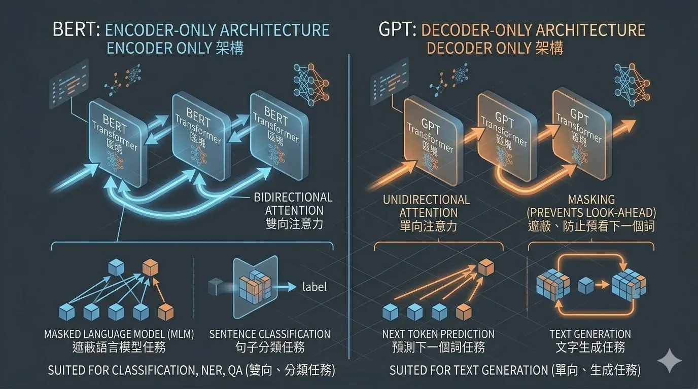
圖4 ▲ BERT（Encoder）雙向看整句話適合分類；GPT（Decoder）單向只看左邊適合文字生成

HuggingFace：幾行程式碼完成推論

前面幾個檔案從零實作 Transformer 是為了理解原理，實際工作中我們用 HuggingFace：

from transformers import AutoTokenizer, AutoModel, pipeline

# 載入 tokenizer 和模型
tokenizer = AutoTokenizer.from_pretrained("bert-base-uncased")
model = AutoModel.from_pretrained("bert-base-uncased")

# 批次 tokenize
texts = ["I love machine learning.", "Transformers changed NLP."]
encoded = tokenizer(
    texts,
    padding=True,
    truncation=True,
    max_length=32,
    return_tensors="pt",
)
# encoded["input_ids"]      → token id 序列
# encoded["attention_mask"] → 1=真實 token，0=padding

# 模型推論
with torch.no_grad():
    outputs = model(**encoded)

# last_hidden_state: (batch, seq_len, 768)
# 每個 token 都得到一個 768 維的向量

最快的方式是用 Pipeline API，直接包好整個推論流程：

# 情感分析
sentiment = pipeline(
    "sentiment-analysis",
    model="distilbert-base-uncased-finetuned-sst-2-english",
)

results = sentiment(["I love this!", "This is terrible."])
# [{'label': 'POSITIVE', 'score': 0.9998}, {'label': 'NEGATIVE', 'score': 0.9997}]

# 文字生成
generator = pipeline("text-generation", model="gpt2")
output = generator("Machine learning is", max_new_tokens=30)

Sentence Embedding 與語意搜尋

BERT 的 CLS token 或 mean pooling 可以把一句話壓縮成一個向量，這個向量代表句子的「語意」：

def mean_pooling(model_output, attention_mask):
    token_embeddings = model_output.last_hidden_state
    mask = attention_mask.unsqueeze(-1).float()
    return (token_embeddings * mask).sum(dim=1) / mask.sum(dim=1)

embeddings = mean_pooling(outputs, encoded['attention_mask'])
# shape: (batch, 768)，每個句子一個向量

# 計算句子相似度
sim = embeddings @ embeddings.T
# 「A dog is running.」和「A puppy is playing.」的相似度 >> 「Machine learning is fascinating.」

這是語意搜尋（Semantic Search）的基礎。

---

小結

概念	重點
Self-Attention	動態計算 token 之間的相關性，Q/K/V 三向量
Multi-Head	多個 head 同時關注不同語言關係，最後合併
Positional Encoding	sin/cos 函式補充位置資訊
BERT vs GPT	Encoder（雙向，分類）vs Decoder（單向，生成）
HuggingFace	AutoTokenizer + AutoModel + Pipeline，快速使用預訓練模型

理解了 Transformer 架構之後，接下來的 Fine-tuning 才會真正有感——我們調整的是已經「懂語言」的模型，讓它學會特定任務，而不是從頭訓練。

---

GitHub

• 完整程式碼：MLOps 學習 repo — phase2